Wednesday, August 31, 2022

What is State in RNN

The “state” of the RNN is reset when processing two different and independent sequences. Recurrent neural networks are a special type of neural network where the outputs from previous time steps are fed as input to the current time step. Basic Recurrent neural network with three input nodes


references:


Sunday, August 28, 2022

Deep Learning - Learning Rate Intro

 The weights of a neural network cannot be calculated using an analytical method. Instead, the weights must be discovered via an empirical optimization procedure called stochastic gradient descent.


The optimization problem addressed by stochastic gradient descent for neural networks is challenging and the space of solutions (sets of weights) may be comprised of many good solutions (called global optima) as well as easy to find, but low in skill solutions (called local optima).


The amount of change to the model during each step of this search process, or the step size, is called the “learning rate” and provides perhaps the most important hyperparameter to tune for your neural network in order to achieve good performance on your problem.


Learning rate controls how quickly or slowly a neural network model learns a problem.

How to configure the learning rate with sensible defaults, diagnose behavior, and develop a sensitivity analysis.

How to further improve performance with learning rate schedules, momentum, and adaptive learning rates.


references:

https://machinelearningmastery.com/learning-rate-for-deep-learning-neural-networks/

What is AUC in Machine learning

AUC provides an aggregate measure of performance across all possible classification thresholds. One way of interpreting AUC is as the probability that the model ranks a random positive example more highly than a random negative example. For example, given the following examples, which are arranged from left to right in ascending order of logistic regression predictions: 

AUC represents the probability that a random positive (green) example is positioned to the right of a random negative (red) example.

AUC ranges in value from 0 to 1. A model whose predictions are 100% wrong has an AUC of 0.0; one whose predictions are 100% correct has an AUC of 1.0.

Positive and negative examples ranked in ascending order of logistic regression score

references:

https://developers.google.com/machine-learning/crash-course/classification/roc-and-auc#:~:text=AUC%20represents%20the%20probability%20that,has%20an%20AUC%20of%201.0.

Wednesday, August 17, 2022

React Widget - Compiling all react files to single file

 https://github.com/facebook/create-react-app/issues/3365


React Widget - Creating React app and embed into single HTML

Great resource this one is

references:

 https://www.labnol.org/code/bundle-react-app-single-file-200514

Tuesday, August 9, 2022

Gradient Descent Explained Simply with Examples

 Introduction to Gradient Descent Algorithm

Gradient descent algorithm is an optimization algorithm which is used to minimise the function. The function which is set to be minimised is called as an objective function. For machine learning, the objective function is also termed as the cost function or loss function. It is the loss function which is optimized (minimised) and gradient descent is used to find the most optimal value of parameters / weights which minimises the loss function. Loss function, simply speaking, is the measure of the squared difference between actual values and predictions. In order to minimise the objective function, the most optimal value of the parameters of the function from large or infinite parameter space are found.

What is Gradient Descent?

Gradient of a function at any point is the direction of steepest increase or ascent of the function at that point.

the gradient descent of a function at any point, thus, represent the direction of steepest decrease or descent of function at that point.

How to calculate Gradient Descent?

In order to find the gradient of the function with respect to x dimension, take the derivative of the function with respect to x , then substitute the x-coordinate of the point of interest in for the x values in the derivative. Once gradient of the function at any point is calculated, the gradient descent can be calculated by multiplying the gradient with -1. 

Here are the steps of finding minimum of the function using gradient descent:

Calculate the gradient by taking the derivative of the function with respect to the specific parameter. In case, there are multiple parameters, take the partial derivatives with respect to different parameters.

Calculate the descent value for different parameters by multiplying the value of derivatives with learning or descent rate (step size) and -1.

Update the value of parameter by adding up the existing value of parameter and the descent value. The diagram below represents the updation of parameter 𝜃 with the value of gradient in the opposite direction while taking small steps.
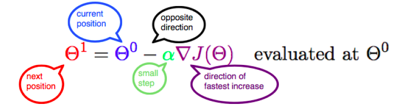
Update the parameter value with gradient descent value

In case of multiple parameters, the value of different parameters would need to be updated as given below if the cost function is 12𝑁∑(𝑦𝑖–(𝜃0+𝜃1𝑥)2) if the regression function is 𝑦=𝜃0+𝜃1𝑥

The parameters will need to be updated until function minimises or converges. The diagram below represents the same aspect.


references:

https://vitalflux.com/gradient-descent-explained-simply-with-examples/


Back propagation in simple terms

Back propagation is an algorithm used in machine learning that works by calculating the gradient of the loss function, which points us in the direction of the value that minimizes the loss function. It relies on the chain rule of calculus to calculate the gradient backward through the layers of a neural network. Using gradient descent, we can iteratively move closer to the minimum value by taking small steps in the direction given by the gradient.


During forward propagation, we use weights, biases, and nonlinear activation functions to calculate a prediction y hat from the input x that should match the expected output y as closely as possible (which is given together with the input data x). We use a cost function to quantify the difference between the expected output y and the calculated output y hat.

The goal of backpropagation is to adjust the weights and biases throughout the neural network based on the calculated cost so that the cost will be lower in the n
ext iteration. Ultimately, we want to find a minimum value for the cost function.


With calculus, we can calculate how much the value of one variable changes depending on the change in another variable. If we want to find out how a change in a variable x by the fraction dx affects a related variable y, we can use calculus to do that. The change dx in x would change y by dy.

In Calculus notation, we express this relationship as follows.


The first derivative of a function gives you the slope of that function at the evaluated coordinate. If you have functions with several variables, you can take partial derivatives with respect to every variable and stack them in a vector. This gives you a vector that contains the slopes with respect to every variable. Collectively the slopes point in the direction of the steepest ascent along the function. This vector is also known as the gradient of a function. Going in the direction of the negative gradient gives us the direction of the steepest descent. Going down the route of the steepest descent, we will eventually end up at a minimum value of the function.
